Introduction
A data series is an ordered sequence of data points. The data can describe a dynamic process, such as the evolution of stock prices; spatial data, like the depth profiles in oceanography; rankings, like in sports competitions; or event logs, like software execution traces. The series fundamentally captures an order, whether it’s on time, space, rank, or another dimension. The sequence is generally called a time series if the order is based on time.
Time series can be found in various applications, from complex systems monitoring machinery performance in industrial environments to everyday medical equipment tracking patient heartbeats. Detecting anomalies in real time within these series becomes critical for saving time, resources, and even lives.
In Digital Sense we have considerable experience working with vast volumes of data and anomaly detection, as demonstrated in our success stories ‘We Increase Ulta’s Marketing ROI with Data Science’ and ‘Best Leather Quality Control with AI-Enhanced Inspection’. Recently, a new project emerged that integrates both lines of knowledge to develop a state-of-the-art solution for real-time anomaly detection in time series.
In this article, we introduce key concepts of anomaly detection in time series and present the solution we developed for a project on the topic.
General concepts
Time series may consist of one or multiple real-valued signals. It is referred to as univariate if it contains only one signal; if it includes multiple signals, it is called multivariate.
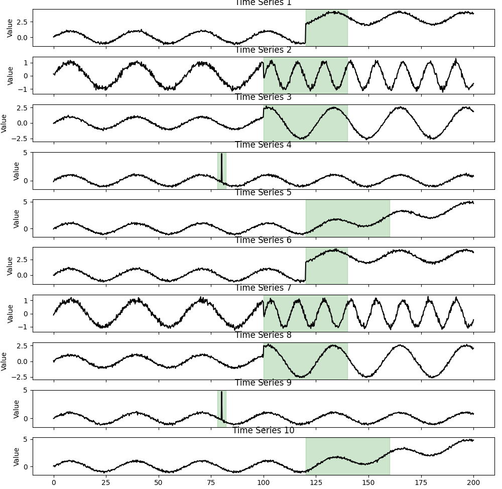
Anomalies in time series can be categorized as point-based or sequence-based, depending on their extent. Additionally, anomalous values may fall either inside or outside the expected healthy range of the series. In some cases, values may lie within normal parameters but still be considered anomalous when analyzed in context. Furthermore, individual signals may appear normal in a multivariate time series when examined separately. However, when evaluated together, specific patterns may emerge that indicate anomalous behavior, revealing dependencies or correlations that would otherwise go unnoticed.
Automatically detecting anomalous behavior enables timely human intervention, accelerating response times and preventing accidents. The algorithms used for this task range from classical approaches, such as k-nearest neighbors, to more advanced methods like diffusion-based models. In practice, no one-size-fits-all solution for anomaly detection in time series exists. The effectiveness of a detection algorithm depends on the characteristics of the time series and the nature of the anomalies. The next section introduces a taxonomy for classifying anomaly detection algorithms, as presented in An Interactive Dive into Time Series Anomaly Detection [1].
Algorithm classification
The first distinction between anomaly detection algorithms is based on the training method used and the availability of labeled data. This classification divides them into supervised, unsupervised, and semi-supervised approaches.
Supervised algorithms categorize data as either normal or anomalous, learning to distinguish between them during training. When presented with a new time series, these algorithms identify anomalous subsequences that match their learned representation of abnormal behavior. However, their main limitation is that they can only detect anomalies similar to those seen during training, making them ineffective in identifying previously unseen anomalies.
In contrast, unsupervised algorithms detect anomalies without prior labeled data and do not require a training phase. These methods assume that anomalies differ from normal data in some way—such as frequency, amplitude, or statistical distribution—which allows them to distinguish anomalies based on inherent differences.
Semi-supervised algorithms fall between these two categories. They require a training phase but are trained exclusively on normal data, learning a representation of expected behavior. When applied to a new time series, any subsequence that deviates from the learned normal pattern is flagged as anomalous.
Another classification of algorithms is proposed in An Interactive Dive into Time Series Anomaly Detection [1], which categorizes them into three main groups based on their approach: distance-based, density-based, and prediction-based methods. Figure 1 shows the proposed classification.
Distance-based methods use distance metrics to compare points or subsequences within a time series. Anomalous subsequences are expected to have more considerable distances from other subsequences than normal ones. Algorithms such as k-means and k-nearest neighbors fall into this category.
Density-based methods estimate the density of the data space and identify anomalies as points or sequences that reside in low-density regions. A notable example is Isolation Forest, which randomly partitions the space and defines anomalies based on the depth of the trees.
Prediction-based methods focus on forecasting or reconstructing a set of time steps using a given context window. The predicted or reconstructed values are then compared to the actual observations, and deviations from the expected values indicate potential anomalies.
This categorization effectively summarizes the main approaches found in the literature. In the following sections, we present a case study and discuss the methods we applied to address the problem.

Case study
Recently, we had the opportunity to apply this knowledge to an industrial client. The client operated several pipelines throughout the plant, each with a flowmeter that continuously measured the flow rate. The data was easily accessible in real-time via API calls. Our task was to analyze this signal and determine whether it exhibited anomalies.
Some of these pipelines had an associated control signal, meaning we were working with a multivariate time series. The degree of correlation between the signals varied: in some cases, the relationship was strong, while in others, it was not immediately apparent through visual inspection. Additionally, some pipelines only had flowmeter data, making those cases univariate time series.
The objective was to design and train an algorithm capable of detecting anomalous behavior in real-time. Moreover, the model needed to handle both univariate and multivariate cases. An initial exploration of the data revealed the presence of multiple types of anomalies. After preliminary testing, we concluded that relying on a single detection method would be insufficient. Instead, we adopted an ensemble approach—an architecture that combines the outputs of multiple algorithms, each based on a different detection strategy. By aggregating these diverse perspectives, the ensemble method offers greater robustness and improved performance compared to any individual model. Figure 2 illustrates an example of how the ensemble method works.

Since the client had to process at least a thousand signals and train an ensemble model for each pipeline, manually labeling data was not feasible. As a result, we opted for semi-supervised and unsupervised algorithms.
Several algorithms were tested to build the ensemble. The final solution combines classical distance-based methods, density-based approaches, correlation measurements, and frequency analysis. Each method was adapted to produce an anomaly score, which was then aggregated to generate the final score, identifying potential anomaly regions within the series.
The next section will outline the complete methodology, from the pre-processing stage to the final score combination.
Ensemble method
To begin with, we retrieve data from the client’s API, which provides both control and flowmeter signals. The API allows us to specify the desired sample rate and the reduction method to apply, in our case, the mean. Once the data is collected, missing values must be handled. In some cases, imputing zero values is sufficient, while linear interpolation provides a more accurate solution in others.
A normal segment of the series should be selected as training data. To ensure its validity, either a visual inspection or a more sophisticated method should be used to identify and confirm a representative normal section. Each algorithm that forms the ensemble is then trained independently with the selected training data.
As explained in the previous section, the algorithms produce an anomaly score during inference. The ensemble integrates these scores and applies a threshold to determine whether the evaluated samples exhibit anomalous behavior.
The combination of anomaly scores remains an open challenge, as different methods can produce varying results, and no universally optimal approach exists. Our approach involved normalizing and rescaling all scores. We then grouped methods based on the type of anomaly they detected, summing and multiplying group results to minimize the risk of missing a detection.
Finally, an anomaly detection threshold must be established. This value can be determined experimentally or set as the 95th percentile of training values. Either way, an alarm should be triggered whenever anomalous behavior is detected.
Conclusion
Real-time anomaly detection in time series provides a critical advantage, enabling swift intervention to prevent accidents, optimize resource usage, and mitigate financial and operational losses. However, handling data with precision is essential, as it drives key decision-making and serves as a foundation for downstream processes, where inaccuracies can have cascading effects.
As discussed throughout this article, no universal approach or single model fits all anomaly detection problems. Instead, each case requires a tailored solution. Our Data Science services has given us extend experience designing and implementing advanced anomaly detection solutions customized to specific needs. Explore our full range of services here to discover how we can help you address your most complex data challenges.
References
[1] Boniol, P., Paparrizos, J., & Palpanas, T. (2024, May). An interactive dive into time-series anomaly detection. In 2024 IEEE 40th International Conference on Data Engineering (ICDE) (pp. 5382-5386). IEEE.
[2] Schmidl, S., Wenig, P., & Papenbrock, T. (2022). Anomaly detection in time series: a comprehensive evaluation. Proceedings of the VLDB Endowment, 15(9), 1779-1797.
[3] Zhang, K., Wen, Q., Zhang, C., Cai, R., Jin, M., Liu, Y., ... & Pan, S. (2024). Self-supervised learning for time series analysis: Taxonomy, progress, and prospects. IEEE transactions on pattern analysis and machine intelligence.


.jpg)