Time Series Analysis with Databricks: A Complete Guide

What is time series analysis and why does it matter?

In high-stakes decision-making, information never sits still. Consumer behaviors shift, markets evolve, and physical assets wear down over cycles. If we analyze this data as a static photo, we miss the movie entirely. Time Series Analysis allows us to capture this motion, modeling dependencies over time to extract value from chaos.

Transitioning from descriptive analytics to true predictive modeling is what separates market leaders from the rest, but it is not a trivial task. It’s not merely about guessing the next number in a sequence; it’s about engineering systems that understand the underlying forces of reality. 

Unlike standard regression problems where data points are often assumed to be independent and identically distributed (i.i.d.), time series data is characterized by autocorrelation. The value of an observation at time $t$ is inherently dependent on previous values ($t-1, t-2, \dots$) and often on the past values of the error terms. This dependency structure means that standard machine learning techniques, if applied blindly, often fail to capture the true dynamics of the system.

From optimizing energy loads on national grids to managing inventory for global retailers, the applications are vast. Yet, as the volume of temporal data explodes—driven by IoT sensors, clickstreams, and real-time transaction logs—traditional modeling approaches struggle to scale. This is where modern architectures like the Databricks Lakehouse become essential, providing the computational throughput to move from analyzing thousands of rows to petabytes of history.

Key components of time series data

To model a time series effectively, one must first understand its anatomy. A raw time series signal is rarely a single, monolithic entity. Instead, it is a composite of several underlying forces. Classical decomposition theory suggests that a series $Y_t$ can be separated into three distinct components:

1. Trend ($T_t$): The long-term progression of the series. This represents the underlying direction (upward, downward, or stable) over a prolonged period, filtering out high-frequency noise. For instance, in an industrial context, this might represent the gradual efficiency loss of a turbine over years of operation.
2. Seasonality ($S_t$): A repeating, predictable pattern over a fixed and known period. This is driven by systemic cycles. In retail, sales spikes in December are a clear seasonal effect. In energy, daily consumption curves follow the sun, peaking during daylight or evening hours depending on the region.
3. Residual/Noise ($R_t$): The stochastic variation that remains after the trend and seasonality are removed. In a theoretically sound model, these residuals should resemble white noise—a sequence of uncorrelated random variables with zero mean and constant variance. If patterns remain in the residuals, the model has failed to capture some aspect of the signal.

‍

Mathematical Composition

These components are typically combined using one of two primary structural models:

• Additive Model: $Y_t = T_t + S_t + R_t$
  
  • Used when the magnitude of the seasonal fluctuations is constant over time (e.g., an increase of 100 units every December, regardless of total sales).
• Multiplicative Model: $Y_t = T_t \times S_t \times R_t$
  
  • Used when the seasonal fluctuations scale proportionally with the trend (e.g., sales increase by 10% every December).

Common techniques used in time series analysis

The field of time series analysis has evolved from classical econometrics to state-of-the-art Deep Learning. At Digital Sense, we employ a "right tool for the job" philosophy, selecting the architecture that balances accuracy with computational efficiency.

Classical Stochastic Models (ARIMA/SARIMA)

For datasets with linear relationships and relatively stable variance, the Box-Jenkins method remains a robust standard.

• AR (AutoRegressive): Regresses the variable on its own lagged (past) values.
• I (Integrated): Applies differencing to make the series stationary (removing trends).
• MA (Moving Average): Models the error term as a linear combination of error terms occurring contemporaneously and at various times in the past.

These models are highly interpretable, making them ideal for financial or regulatory environments where explaining why a forecast was made is as critical as the forecast itself.

Modern Deep Learning Approaches

However, many real-world enterprise problems involve non-linear dependencies and high-dimensional data (multivariate series). In these cases, we utilize neural network architectures:

• LSTMs (Long Short-Term Memory): A type of Recurrent Neural Network (RNN) capable of learning long-term dependencies. Unlike standard RNNs, which suffer from the vanishing gradient problem, LSTMs maintain an internal "cell state" that can carry information across many time steps, making them effective for sequences where an event at $t-100$ might influence $t$.
• Transformers: Originally designed for Natural Language Processing, Transformer-based models (such as the Temporal Fusion Transformer or TFT) are now achieving state-of-the-art results in forecasting. They utilize attention mechanisms to dynamically weigh the importance of different time steps, allowing the model to focus on specific past events that are relevant to the current prediction.

Why use Databricks for time series analysis?

Developing a forecasting model on a local laptop is fundamentally different from operationalizing it at an enterprise scale. Organizations often struggle with fragmented data silos—historical logs in a data lake, customer data in a warehouse, and real-time streams in a message bus. Databricks solves this by providing a unified Lakehouse architecture.

1. Unified Governance with Unity Catalog

In regulated industries like finance and energy, you must know exactly what data was used to train a model. Databricks Unity Catalog provides a centralized governance layer for both data and AI assets. It tracks lineage automatically, meaning you can audit a specific model version and trace it back to the exact tables, columns, and notebooks used to create it. This governance is essential for compliance and reproducibility.

2. Massive Scalability with Apache Spark

Time series datasets in the IoT era can grow to billions of rows. A single-node Python script (using pandas) will crash when processing terabytes of sensor data. Databricks is built on Apache Spark, which allows for distributed processing. You can train a single model on a massive dataset, or more commonly, train thousands of models in parallel (e.g., one model per store for a retailer with 5,000 locations) using Spark's distributed compute power. This "many-models" pattern is natively supported and highly optimized on the platform.

3. The Collaborative Lifecycle

Silos between teams kill AI projects. Often, data engineers build pipelines in one tool, while data scientists model in another, leading to "handover" friction. Databricks allows both personas to work in the same workspace. Engineers can build ETL pipelines that feed directly into the Feature Store, which scientists then consume for training, all tracked via MLflow. This seamless integration significantly accelerates the time-to-production.

Setting Up a Time Series Workflow in Databricks

Establishing a production-grade forecasting pipeline requires a structured approach to data engineering and model lifecycle management. At Digital Sense, we typically architect these workflows following the Medallion Architecture, ensuring data quality at every stage before modeling begins.

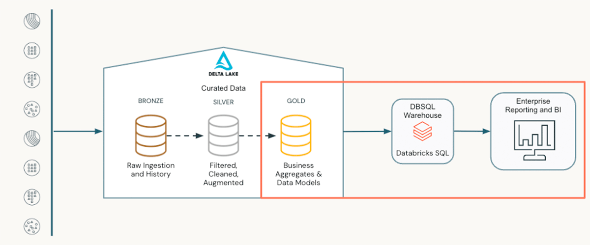
Phase 1: Ingestion and Storage (Delta Lake) The foundation of any time series workflow is Delta Lake. Raw telemetry or transaction logs are ingested into a "Bronze" layer.

• Why it matters: Delta Lake provides ACID transactions and, critically for time series, Time Travel. This allows engineers to query the state of the data as it existed at a specific moment in the past, enabling reproducible experiments and accurate backtesting without needing to snapshot database copies manually.

Phase 2: Temporal Feature Engineering (Feature Store) Once data is cleaned (Silver layer), the challenge is transforming timestamps into predictive signals. This is where the workflow deviates from standard ML.

• The "As-Of" Join: Instead of creating ad-hoc features, we register temporal features (like rolling averages or lag windows) in the Databricks Feature Store. The critical step here is using Point-in-time joins. When generating training sets, the Feature Store automatically joins features based on the event timestamp, ensuring the model never "sees" future data during training—solving the pervasive "Look-Ahead Bias" problem.

Phase 3: Model Training Strategy Depending on the granularity required, the workflow branches into two paths:

• Path A: Rapid Baseline (AutoML): For quick exploration, we trigger Databricks AutoML. It acts as a "glass-box" solution that automatically tests ARIMA, and regression models, handling seasonality and missing data. It outputs editable source code, allowing engineers to refine the best candidate rather than starting from scratch.
• Path B: Fine-Grained Forecasting (Spark + Prophet): For massive scale, such as forecasting 50,000 Stock Keeping Unit (SKUs), we implement a distributed pattern using Spark Pandas user-defined function (UDFs). This splits the data by series ID and trains thousands of lightweight models in parallel across the cluster nodes.

Phase 4: Operationalization (MLflow) The final step is deployment. All experiments, parameters, and metrics are logged automatically in MLflow. The best model is registered and can be deployed via Model Serving for real-time inference or scheduled as a batch job to write forecasts back to a "Gold" table for dashboards.

‍

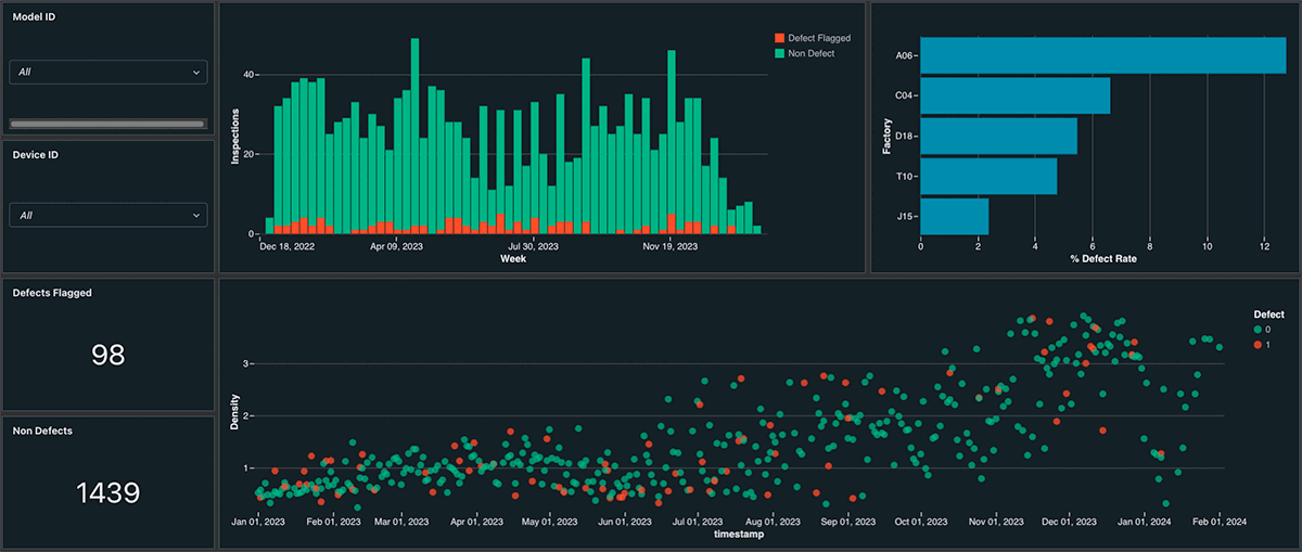
Dashboard visualization example - From Databricks

‍

Best practices for working with time series data analysis

To ensure reliability in production, engineering teams should adhere to rigorous standards:

• Walk-Forward Validation: Never use random k-fold cross-validation for time series. Random shuffling destroys the temporal order. Instead, use Walk-Forward Validation (or rolling-window evaluation), where the model is trained on a past window and tested on a future window, sliding this window forward in time. This simulates the actual forecasting environment.
• Handling Missing Data: Real-world data is messy. Sensors fail; logs drop. Unlike tabular data where rows can be dropped, a missing timestamp breaks the frequency of a time series. Advanced imputation techniques—such as linear interpolation or spline imputation—must be used to fill gaps without introducing bias.
• Monitoring for Concept Drift: The world changes. A model trained on 2019 data would fail in 2020 due to the structural break caused by the pandemic. Continuous monitoring is essential. We implement Databricks Lakehouse Monitoring to detect shifts in the statistical properties of the input data (Concept Drift) or the target variable (Label Drift), triggering automated retraining pipelines when performance degrades.

How Digital Sense helps you accelerate time series projects

Moving from a theoretical understanding of time series to a deployed, scalable solution requires deep technical expertise. 

A prime example of our research-driven approach is our collaboration with UTE (National Administration of Power Plants and Electrical Transmissions). The project involved clustering customers based on behavioral consumption patterns and implementing multivariate forecasting models to estimate future energy demand. By testing state-of-the-art architectures across various time horizons and integrating them into a scalable pipeline, we helped enhance the precision of load estimations—critical for both grid stability and financial planning.

‍

We do not simply apply off-the-shelf algorithms; we engineer solutions using best-in-class infrastructure like Databricks to ensure your predictive intelligence is robust, scalable, and profitable.

FAQs about time series analysis

Q1: What is the difference between time series analysis and standard regression?

Standard regression assumes that data points are independent (e.g., predicting house prices based on square footage). Time series analysis assumes that data points are dependent on previous values (autocorrelation). This requires specialized techniques (like ARIMA or LSTMs) to capture the temporal dynamics that standard regression misses.

Q2: How much historical data do I need for accurate forecasting?

This depends on the complexity of the signal and the seasonality. As a general heuristic, you need enough history to capture at least 2 to 3 full cycles of the pattern you are trying to predict. For example, if you are modeling yearly seasonality, you ideally need 3 years of data. For deep learning models, the data requirements are significantly higher to avoid overfitting.

Q3: Can Databricks handle real-time time series forecasting?

Yes. Databricks supports Structured Streaming, allowing you to ingest and process time series data in real-time. With Model Serving, you can deploy your trained forecasting models as REST endpoints, providing sub-second predictions for use cases like fraud detection, dynamic pricing, or real-time anomaly detection in industrial sensors.

References

1. Digital Sense. (2025). Detecting Anomalies in Time Series: Theory Meets Practice. Retrieved from https://www.digitalsense.ai/blog/detecting-anomalies-in-time-series
2. Databricks. (2025). Databricks AutoML for Time-Series.
3. Databricks. (2025). Time Series Forecasting With Prophet And Spark. Databricks Blog.
4. Microsoft Learn. (2025). Overview of forecasting methods in AutoML. Azure Machine Learning.
5. Box, G. E. P., Jenkins, G. M., Reinsel, G. C., & Ljung, G. M. (2015). Time Series Analysis: Forecasting and Control (5th ed.). John Wiley & Sons.