Tech

Forecasting Electricity Consumption: Same Energy, Different Goals

Published on

May 7, 2026

Introduction

Every machine learning project starts with a dataset. But before any model is trained or any pipeline is built, the most important question to ask is: what does the client actually want?

This is a question that shouldn't be underestimated as answering it defines a comprehensive workflow for the project: plausible forecasting horizons, prediction granularity, relevant covariates, evaluation metrics, and ultimately, which model architecture makes sense. Getting this wrong can be a critical failure. In the energy sector especially, bad predictions carry real operational and financial consequences.

This article walks through the end-to-end process of building an electricity consumption forecasting system for a national utility company, from problem definition to model selection and delivery. The dataset covers hourly smart meter measurements from approximately 150,000 residential and 15,000 non-residential customers. Rather than jumping straight to the models, we start where every forecasting project should: deepening the understanding of what the client actually needs.

Three Clients, Three Perspectives

Consider three interested parties belonging to different departments within the same electrical energy company.

The first works in the grid operation department and is concerned about demand spikes during heat waves. Their interest is highly dependent on temperature covariates, focusing on short-horizon, peak-sensitive predictions. Average accuracy matters far less than reliably predicting anomalous consumption peaks. Missing a spike is costly; a false alarm is manageable.

The second works in the sales department and wants to quantify monthly revenue by tariff segment. This client needs an aggregate, medium-horizon solution that answers: how much energy will each customer category consume over the next month? The approach here is not to capture a single extreme event, but to improve average accuracy across each day within a month. The model needs consistency, not reactiveness.

The third works in infrastructure and is interested in adapting the electrical grid to new consumer behaviour. Since infrastructure upgrades are costly, they need to be planned for the long run. The best approach here is to generate plausible consumption scenarios five to ten years into the future, provided the available data supports it.

Each scenario requires a different approach. As covered in Time Series Data: Analysis vs Forecasting Explained, the nature of the objective also determines how the project's time should be allocated; whether the focus belongs on analysis or forecasting. In the heat wave scenario, for instance, data on these events is scarce by definition, which means forecasting models will not reliably capture their patterns on their own. Analysis paired with domain expertise is needed to correctly incorporate peak behaviour into the model. The same constraint applies to the infrastructure case: the ratio of available historical data to the required prediction horizon can be extremely unfavourable, which fundamentally limits what a pure forecasting approach can deliver.

What our client needed

The project described in this article maps most closely to the second and third scenarios, but with a broader mandate. The client needed a system capable of forecasting electricity consumption across multiple horizons: the next day, the next week, and the next month. Predictions were to be generated within clusters defined by tariff type and geographic region for residential customers, and by tariff alone for non-residential ones.

Now, the client was also interested in exploring electricity demand under different conditions: consumption variation depending on temperature fluctuations, and, also, how regional load shifts depending on the season. This pushed the solution beyond standard forecasting into scenario simulation and the development of a tool that makes that exploration accessible.

Data Preparation: Aggregation, Covariates, and Normalization

Technical decisions made before any model is trained often determine more of the outcome than the model choice itself. Three areas deserved particular attention during the project.

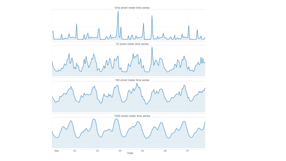
Spatial and temporal aggregation involves a fundamental trade-off. Training models on individual smart meter time series preserves granularity but introduces significant noise into predictions since the model must account for variability across individual clients. When the task involves forecasting aggregated cluster-level consumption, it is often more pragmatic to train directly on the aggregated series across all meters belonging to a cluster. Aggregated series also tend to be more predictable: individual consumption behaviour is erratic, but at the cluster level, structured patterns emerge that models can learn from reliably. However, this comes at a cost: with ~150,000 individual meters collapsed into 20–24 aggregated series, the model must generalize from far less data. There is also a structural limitation worth noting, as a model trained at a given aggregation level cannot produce predictions at a finer one. If versatility across granularities is a requirement, aggregation may not be your best friend.

‍

Covariates divide into two categories with different treatment. Static covariates like tariff type or geographic region describe fixed characteristics of a series and can be encoded directly. Dynamic covariates change over time and require forecasts of their own as inputs: temperature projections, holiday calendars, and time-of-week indicators are the most impactful in electricity consumption. Crucially, this information must also be provided for future predicted dates, not only for the historical window. Not all model architectures incorporate dynamic covariates natively, though different workarounds exist that allow for their inclusion.

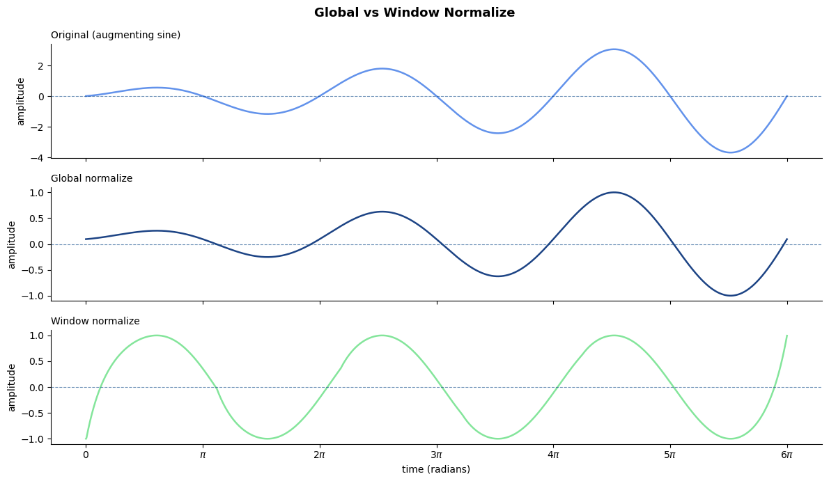
Normalization determines how each time series input is scaled before being fed into the model, directly affecting what the model learns to represent. Global normalization preserves relative magnitudes across series, which matters when the model needs to distinguish high-consumption regions from low-consumption ones. On th oither hand, window-based normalization, teaches the model the shape of consumption patterns but loses magnitude context. For electricity consumption, window-based normalization is generally the default and a good way to go, as it reduces bias toward high-consumption clusters. Temperature data, however, benefits more from global normalization: the absolute value carries meaningful information, since how people perceive heat and adjust their consumption depends on the actual temperature, not just its relative shape within a window.

‍

Choosing the Right Model and Loss

The landscape of available models goes from statistical methods like ARIMA and Prophet, to gradient boosting approaches like LightGBM, to deep learning architectures including Transformers, RNNs, and MLP-based models. A thorough treatment of the state of the art is available in Time Series Forecasting: A Deep Dive into the State of the Art and Current Trends. But architecture performance benchmarks are only one input into the model selection decision.

A frequently underestimated dimension is how each model structurally handles covariates. Some architectures integrate dynamic covariates natively into their prediction mechanism, meaning external information like temperature or holiday flags shapes the output directly. Others treat covariates as secondary inputs or require engineering workarounds that could dilute their meaning.

There is also the question of whether it would be more useful to train models globally, meaning training it across all series associated with different clusters, or to train individual models, each associated with one cluster separately. For global models, when series share structure, their commonalities can be exploited by the model improving the overall performance.This also enables the usage of more complex models, since there is more data available. For individual models, they tend to capture series specific dynamics but require sufficient data per series to generalize. In our case, since each series is distinct enough to warrant its own specialized model, individual models were used.

There is also the question of whether to train a single global model across all cluster associated series, or individual models, each specialized for one cluster. Global models can benefit from shared structure across series, improving overall performance when commonalities exist. Also, it enables the use of more complex architectures since more data is available. Individual models, on the other hand, capture series-specific dynamics but require sufficient data per series to generalize. In our case, each cluster series is distinct enough to warrant its own specialized model, so individual models were the natural choice.

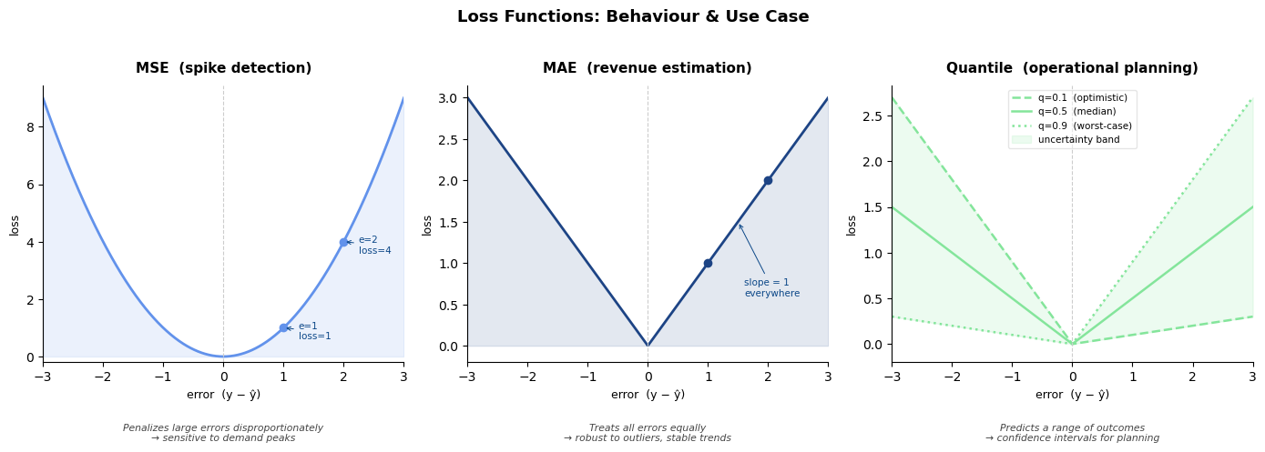
The loss function is the final major lever, and it should follow directly the client's objective:

MSE penalizes large errors disproportionately, making it sensitive to demand peaks, making it appropriate when spike detection is the priority.
MAE treats all errors equally, producing stable trend predictions robust to outliers better suited for revenue estimation.
Quantile loss trains the model to predict a range of outcomes rather than a single value, enabling confidence intervals that quantify uncertainty, making it great for operational planning where worst-case scenarios matter as much as expected values.

‍

What We Built: The Solution Delivered

The project involved forecasting electricity consumption for a national utility company working with smart meter data from approximately 150,000 residential and 15,000 non-residential customers, covering August 2022 to August 2025 (excluding the pandemic period to ensure representative consumption patterns).

After aggregating meters into regional and tariff-based groups, resulting in twenty time series for residential and four for non-residential, the team selected the Mixture of Linear Experts with Residual MLP (MoLE-RMLP) architecture. Even though the model did not natively support dynamic covariates, the team worked to adapt it. This model represents a good compromise between the amount of data available and its complexity. Its "mixture of experts" mechanism activates different components of the network depending on external conditions: for example, one set of experts learns summer high-temperature patterns while another specializes in winter demand behavior, which structurally fits into the problem elegantly.

The full pipeline incorporates two key covariate types: hourly temperature variation data from national meteorological stations (applied to residential customers) and a holiday indicator alongside standard temporal features. Data is subsampled according to the prediction horizon used: for daily predictions, hourly data is used, for weekly predictions, data is subsampled to six hours by adding consecutive six hour meter samples. For monthly predictions, data is subsampled to a day.

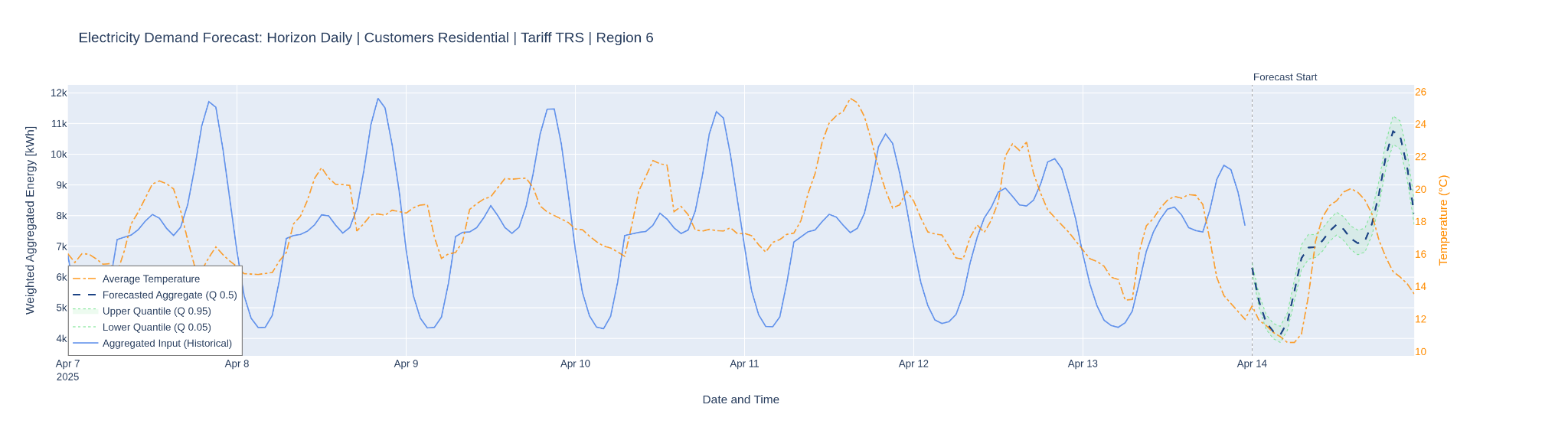
Confidence intervals are generated via quantile loss, which means training three parallel outputs: the 5th percentile, which attempts to predict the lowest plausible consumption value (in only 5% of cases does the actual value fall below it); the 95th percentile, which attempts to predict the highest plausible value (in 95% of cases the actual value falls below it); and the 50th percentile, which behaves similarly to minimizing mean absolute error, penalizing over- and under-prediction equally and producing the central estimate.

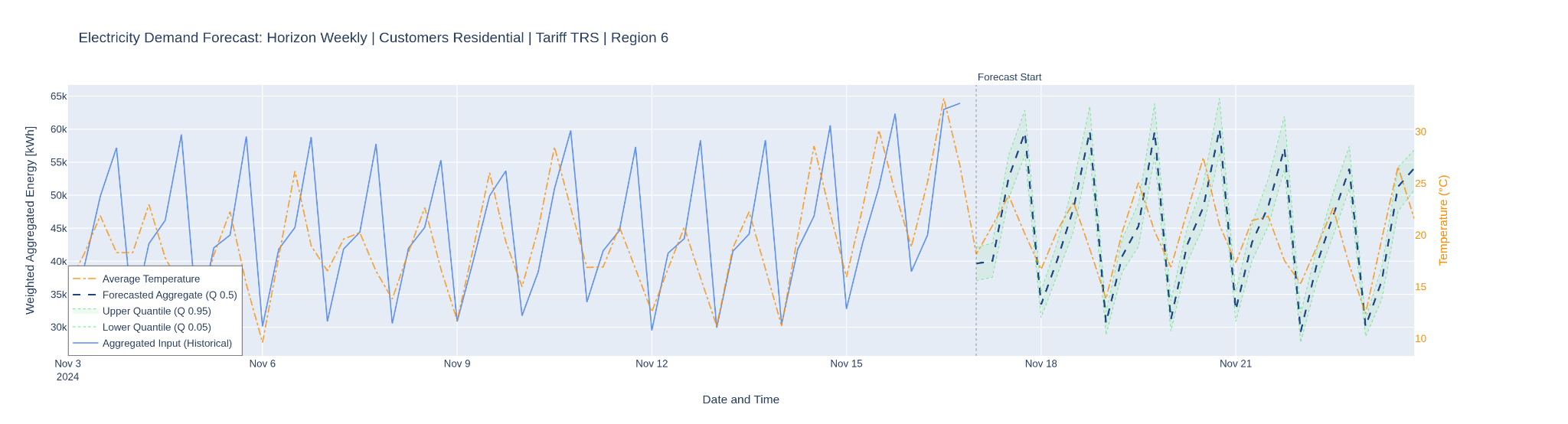
Electricity Demand Forecast: Horizon Weekly

Here the results validate the approach. Residential MAPE reached 2.7% at daily prediction horizon, 3.2% at weekly, and 8.8% at monthly, in each case outperforming the baseline (naive repetition of the last observed period) by a substantial margin. Non-residential results reached 5.5% weekly and 6.9% monthly. Critically, the inclusion of temperature and holiday covariates reduced error by up to 50% relative to models trained without them, a finding that underscores just how much predictive power lies in external information when the model is designed to use it properly.

Electricity Demand Forecas: Horizon Daily

‍

Conclusion

The most important aspect of this project was asking the right questions before selecting any model. What does the client actually need to know? Over what horizon? How will the predictions be used? What events most affect consumption, and how often do they occur in the data?

Each of these answers shapes a different set of technical decisions on aggregation, covariate design, architecture, and loss functions. When those decisions are made in service of the actual objective, the results speak for themselves.

If your organization is working on energy demand forecasting, or any problem where prediction needs to be operationally useful get in touch with Digital Sense. We bring research-driven rigor and a track record of delivering production-ready solutions to the problems that matter.