Workforce Scheduling and Routing: Choosing the Right Optimization Method

Published on

November 4, 2026

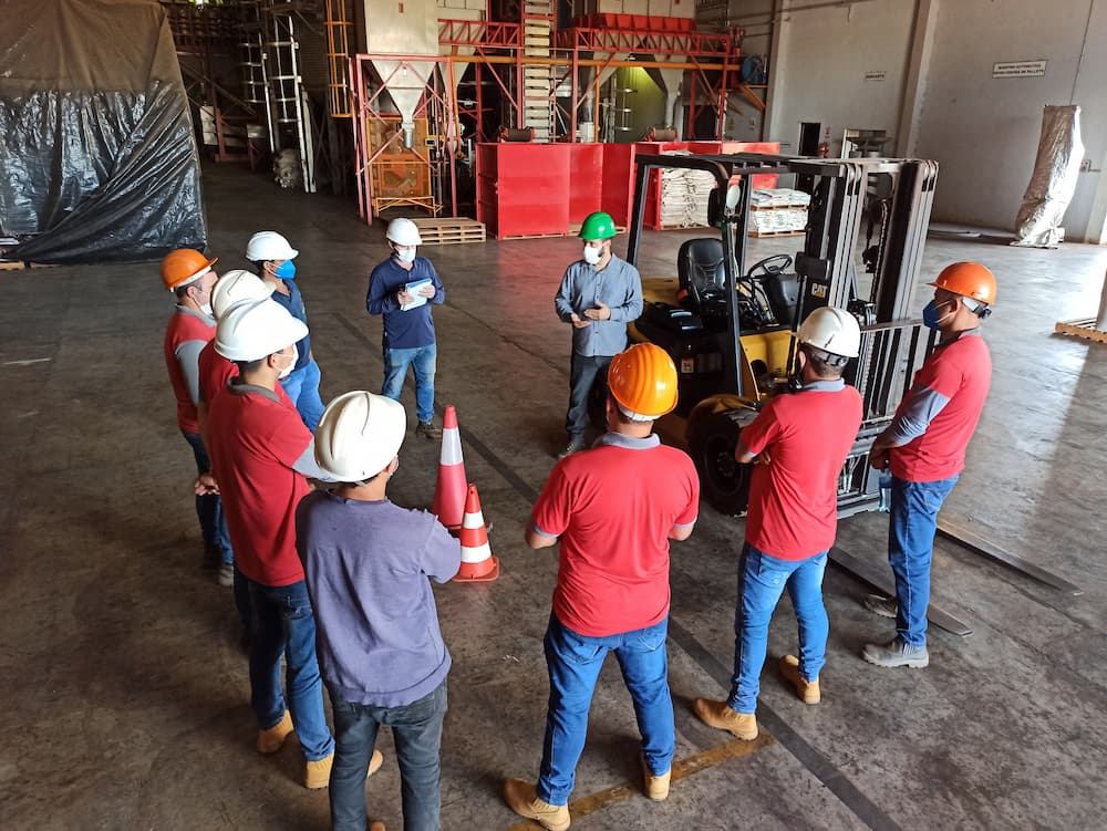
Everyone who has worked and managed a workforce (technicians, maintenance crews, field service teams) knows that scheduling and routing across multiple locations is a challenge shared by many industries, yet it is often handled through experience alone.

This article introduces the Workforce Scheduling and Routing Problem (WSRP), showing how it builds on simpler, well-known optimization problems to form a richer problem that captures skills, time windows, and logistics. We then walk through the main families of solution methods (exact, metaheuristic, matheuristic, and reinforcement learning approaches), comparing their strengths and trade-offs to help decide which one fits a given scheduling challenge.

‍

Introduction

For many industries, core operations depend on scheduling tasks across multiple locations with a limited workforce and resources. For example, O&M teams have to perform preventive and corrective maintenance on different sections of an industrial plant; healthcare providers must attend both emergency calls and non-emergency home visits; commercial services (e.g., pest control providers) must visit various clients and perform different tasks depending on each individual case.

Several companies rely on their workforces’ expertise to generate the schedule. However, the number of decision variables (e.g., worker assignment and route selection) often makes this planning step very complex, and relying solely on experience might leave room for improvement. In addition, external factors such as sudden weather changes or unexpected events might disrupt the existing plan and force the team to act fast and update the schedule accordingly.

A more systematic way to generate such a schedule is to apply modeling and numerical optimization techniques. The field that analyzes such problems is known as Operations Research (OR) [1]. Within this field, this class of problems is known as a Workforce Scheduling and Routing Problem (WSRP).

In this article, we analyze the WSRP in detail. In the first subsection, we describe how the problem builds up from a series of simpler ones, then examine variations within WSRP itself. In the second section, we present and compare various numerical solution approaches for finding optimal or near-optimal schedules. Finally, in the last section, we present some conclusions and recommendations for solving a problem of this nature.

Problem variations

In the OR literature, problems are categorized based on their complexity and modeling assumptions. In general terms, there are two key decision structures that often appear in problems of this nature: assignment and routing. In the former, the goal is to find a one-to-one matching between n tasks and m agents, aiming to minimize the total assignment cost [4]. In the latter, the goal is to find an optimal set of routes to execute a list of tasks [5]. From these starting points, several well-studied problems were defined.

Complexity increase

One of the first ones was the Traveling Salesperson Problem (TSP), which tackles the following situation: Given a set of n cities and the distance between them, the goal is to make a complete tour of all cities and back to the starting point, passing through them only once, while covering the shortest distance possible [6]. This problem is purely about routing because there is only one salesman available to perform the required work.

‍

Even the TSP, the simplest variant in this list, is classified as an NP-hard problem, a category in computational complexity theory for problems where the effort required to find an exact solution grows exponentially with the number of cities. Finding an exact solution to NP-hard problems is therefore impractical beyond a fairly small scale. This difficulty carries over to every problem built on top of the TSP.

‍

If we add a fleet of vehicles to the TSP, it becomes the Vehicle Routing Problem (VRP). Here, the objective is to design optimal delivery routes from a central depot to a set of spatially distributed customers, subject to various constraints (e.g., maximum load per vehicle) and given multiple available units [7]. The VRP not only requires taking routing into account, but also assignment, as each vehicle in the fleet is responsible for a specific route. One relevant extension to the VRP is the inclusion of time windows, so that each customer must be served at a specific time. This variant is known as the Vehicle Routing Problem with Time Windows (VRPTW).

‍

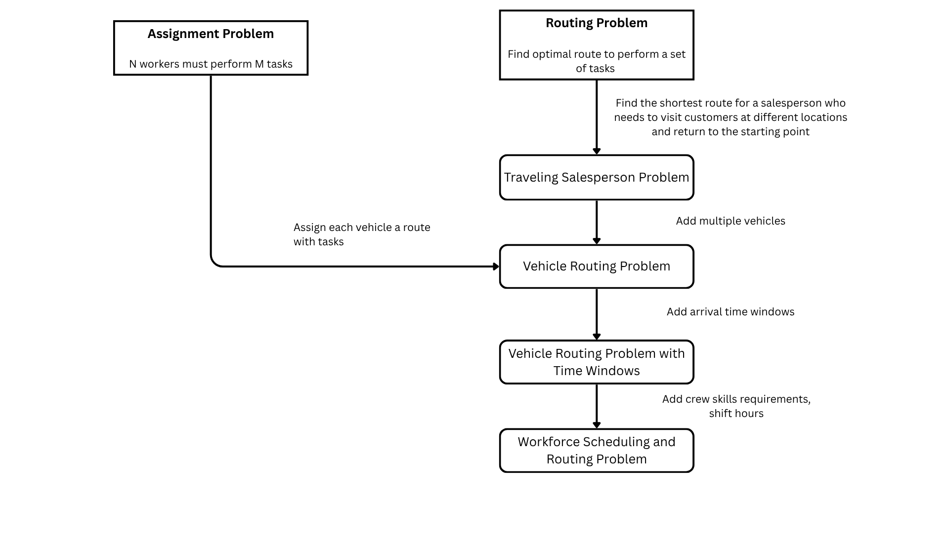
Finally, if we move from delivery to other tasks that require specific skills, with a crew of specialists so that each task is executed by a particular member, we arrive at the Workforce Scheduling and Routing Problem (WSRP). Figure 1 illustrates the progression from the TSP to the WSRP and how each layer adds new assumptions.

‍

*Figure 1: Building blocks of workforce scheduling and routing: Each arrow adds one modeling assumption.*

‍

Variants within WSRP:

WSRP is not a standardized problem. However, it usually has the following characteristics [2]:

Personnel mobilization across different sites and multi-location visits: The workers must move between locations to perform various tasks and usually visit more than one site in a single shift.

Task time windows: the plan must be executed within a specific time frame, and limitations arising from external conditions, such as weather, may be taken into account.
Variable start and end points for personnel: Workers might have different starting points, e.g., start their workday at different offices.
Personnel skills and qualifications: workers might be fit for different tasks
Teaming: When tasks require multiple workers together, fixed teams can be treated as a single unit, but teams that change by task require synchronizing workers' arrival times and re-verifying skill coverage for each new task.
Variable transportation modalities: In some cases, different transportation methods might be needed, e. g., trucks for heavy equipment and cars for personnel.
Resource heterogeneity: speed, capacity limits, operating conditions.
Service duration variability: The time required to complete a task can vary by worker and task type; when durations are long enough that a worker can only complete one task per shift, the problem reduces to task allocation.
Connected activities: Some tasks depend on others; one may need to happen before/after another (sequential dependency), start at the same time (synchronization), overlap, or respect a minimum/maximum time gap from a related task's completion.
Clusterization: Tasks or workers may be grouped by geography, either to limit travel distance, respect territorial assignments, or reduce problem size by solving smaller sub-problems.

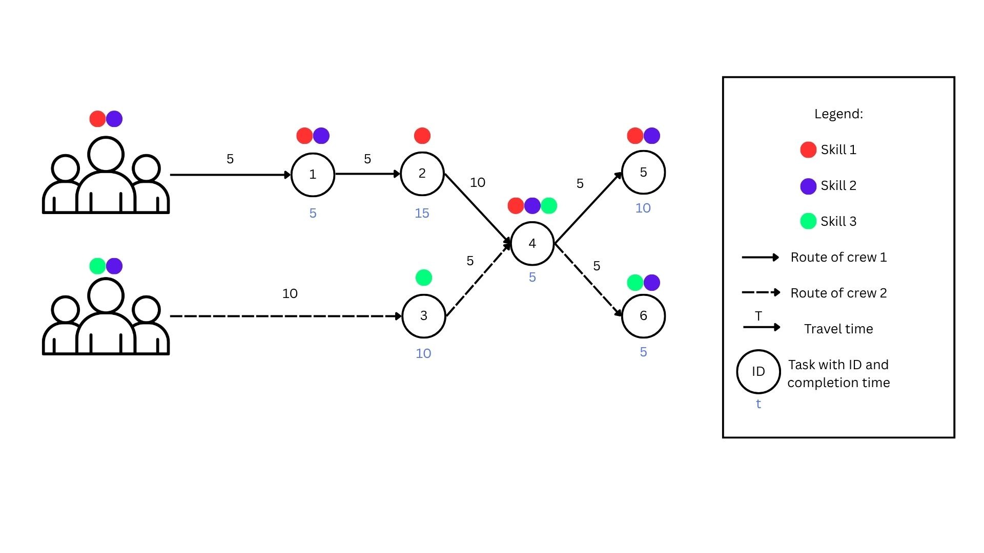
Figure 2 shows an example of a WSRP consisting of two crews, who perform two different routes and execute a total of 6 tasks. As illustrated, the top crew possesses two skills, represented by the red and purple dots, and the bottom crew has the green and purple skills. Therefore, teaming is required to execute task 4.

*Figure 2: Illustrative example of a Workforce Scheduling and Routing Problem with 2 crews, 3 skills, and 6 tasks, adapted from [3].*

‍

Dynamic dimension:

One further aspect of scheduling and routing problems is how to adjust when something unexpected occurs. There are several reasons why a plan might be invalidated, such as adverse weather, a vehicle breakdown, an absent employee, or a task simply running longer than expected. When this happens, the plan must be revised, either by locally repairing the affected routes or by re-optimizing from the current state [8]. These scenarios are commonly known as dynamic routing problems [9].

There are two different approaches to solving a dynamic routing problem: periodic reoptimization and continuous reoptimization. Periodic reoptimization builds an initial plan and then updates it as new data emerges or after a fixed amount of time. Continuous methods, on the other hand, run constantly in the background using an adaptive memory of alternative solutions, so the search can adapt to new data without needing to restart from scratch [3].

When working on a specific WSRP, both the assumptions about the system (e.g., crew, skills, tasks) and its behavior (dynamic or static) must be defined and thoroughly modeled. This step is crucial for applying numerical solution strategies to find an optimal solution, which is covered in the following section.

Solution approaches

Given that WSRP isn't a standardized problem, its definition shifts depending on which constraints and variants a given case includes. Because of that, the solution methods applied to it in the literature aren't standardized either; different papers name and combine them differently depending on the specific variant they tackle. That said, across the literature, the most commonly cited approaches fall into three broad families, plus an emerging fourth: exact methods, metaheuristics, matheuristics, and reinforcement learning.

Exact methods (MILP / CP)

The most direct approach is to see the problem as a Mixed-Integer Linear Program (MILP) and hand it to a solver. These methods have one major strength: when they finish, they guarantee the solution found is truly optimal (or report a bounded gap to optimality), and every constraint in the model is transparent and auditable, so that a decision-maker can trace exactly why a given technician was assigned to a given task.

The thing with this is scalability. WSRP is NP-hard, and the number of decision variables grows quickly with the number of technicians, tasks, and time periods. Solving a full multi-day, multi-technician schedule from scratch with an exact solver can take too long. In practice, exact methods are most competitive when the scope is bounded, a single route, a single day, or a small reoptimization after a minor disruption, rather than the full rolling-horizon problem.

Heuristics/Metaheuristics

When the problem is too large for an exact solver to handle in a reasonable time, the field turns to heuristics or, more commonly, metaheuristics, general-purpose search frameworks that trade the optimality guarantee for speed and scalability. Several exist (tabu search and genetic algorithms are common alternatives), but the most popular in the routing and scheduling literature specifically is Adaptive Large Neighborhood Search (ALNS) [10].

‍

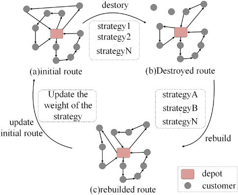
The idea behind ALNS is iterative: start from a feasible (even if poor) schedule, then repeatedly destroy part of it (removing a set of tasks from their current assignment) and repair it by reinserting those tasks, ideally in a better configuration. Every step of this process, including the repair step, is performed using a heuristic rule (e.g., "insert this task at its cheapest available position") rather than an exact solution; nothing in a pure ALNS run guarantees optimality. What makes it "adaptive" is that it keeps several destroy and repair operators on hand and, as the search progresses, learns which ones tend to produce better results, giving them more weight over time.

It’s true that ALNS doesn't guarantee optimality, but it does produce solutions quickly and is suited to repairing an existing schedule rather than rebuilding it from nothing. This is why it's the dominant metaheuristic for the reactive side of the problem described in Section 2: when a new task arrives, or a technician becomes unavailable, ALNS can patch the current plan.

‍

A mixed approach: matheuristics

Exact methods and metaheuristics sit at two different sides of the table: one guarantees quality but doesn't scale, the other scales but gives up the optimality guarantee entirely. Matheuristics are a mixed approach that puts an exact component inside an otherwise heuristic method, so the result is neither purely one nor the other.

Matheuristics can be built in several ways, depending on the problem; there is no single fixed recipe for combining the exact and heuristic sides. A concrete example is [2]: instead of running a single ALNS search, the method runs several ALNS searches in parallel, with each contributing candidate technician tours to a shared pool as it searches. This part is still purely heuristic, same as a standalone ALNS run. What makes it a matheuristic is the next step: that pool of candidate tours is small and structured enough that a mathematical programming method can solve it exactly, selecting the best possible combination of tours from everything the parallel ALNS searches produced. The heuristic side does the work of narrowing an intractably large problem down to a manageable set of good candidates; the exact side then guarantees the best possible choice within that reduced set.

Reinforcement learning

Reinforcement learning (RL) takes a fundamentally different approach: instead of designing rules or search operators by hand, an algorithm learns a decision-making policy by trial and error, receiving a reward signal (e.g., lower cost, fewer late tasks) and adjusting its behavior over many simulated episodes until it gets better at making good decisions on its own. In the broader routing and scheduling literature, this has begun to appear as a way for a system to learn to prioritize or sequence tasks directly from data, rather than following a fixed heuristic rule.

In principle, this kind of approach is appealing for the dynamic case, a well-trained policy can react to a new task or disruption almost instantly, since it doesn't need to re-run an optimization from scratch. In practice, it's still an immature choice for this kind of problem overall. Training a policy requires large amounts of representative data or a realistic simulator, along with significant tuning effort, which is a heavier upfront investment than either of the other approaches. More importantly, a learned policy is a black box: it's much harder to audit or guarantee that it will respect hard, safety-relevant constraints (a technician's certification, a mandatory time window) than it is for an exact or even a metaheuristic solution, which can be explicitly checked.

Overall comparison

No single method wins on every dimension; the right choice depends on the problem's scale and how much the plan needs to react to change.

Dimension	Exact (MILP/CP)	Metaheuristics (ALNS)	Matheuristics	Reinforcement Learning
Solution quality	Optimal (or bounded gap)	Near-optimal, no guarantee	Near-optimal, tighter than pure metaheuristics	Variable, depends on training quality
Solving time	Grows fast with problem size	Fast, predictable	Slower than pure ALNS, faster than pure exact	Very fast once trained
Scalability	Poor for large/full-horizon instances	Good, scales to large instances	Moderate	Good, once trained

Conclusion

The decision to send a crew from one site to the other isn’t arbitrary and can have major impact. Do it right and you will find that idle time shrinks, disruptions are absorbed rather than cascading, and hidden capacity comes to light. On the other hand, do it wrong, or leave it to experience alone, and those same costs quietly compound day after day. This is exactly why the Workforce Scheduling and Routing Problem sits at the center of operational performance.

What this article tries to show is that there's no single "correct" way to solve it. The right method depends on how the operation actually behaves: how large it is, how often plans need to change, and how much time there is to compute an answer. That flexibility allows for a custom solution to be built to fit the specific shape of a real operation, rather than forcing that operation into a generic template.

Getting there though, requires both, knowing the theory, and having an engineering team that can translate an operation's real constraints into a working model, validate it against real data, and fold it into day-to-day decisions. If that's a gap your organization is facing, we’re here to close it, so if you’re interested don’t hesitate to contact us.

‍

References

[1] Carter, M. W., Price, C. C., & Rabadi, G. (2000). Operations research: a practical introduction (p. 416). Boca Raton: Crc Press.

[2] Castillo-Salazar, J. A., Landa-Silva, D., & Qu, R. (2016). Workforce scheduling and routing problems: literature survey and computational study. Annals of Operations Research, 239(1), 39-67.

[3] Demiray, O., Tolga, D., & Yücel, E. (2026). An optimization framework for a dynamic multi-skill workforce scheduling and routing problem with time windows, synchronization constraints, and anticipated tasks. Computers & Industrial Engineering, 112203.

Potential images to add

[4] Pentico, D. W. (2007). Assignment problems: A golden anniversary survey. European Journal of Operational Research, 176(2), 774-793.

[5] Toth, P., & Vigo, D. (Eds.). (2002). The vehicle routing problem. Society for Industrial and Applied Mathematics.

[6] Fenoaltea, E. M., Baybusinov, I. B., Zhao, J., Zhou, L., & Zhang, Y. C. (2021). The stable marriage problem: An interdisciplinary review from the physicist’s perspective. Physics Reports, 917, 1-79.

[7] Laporte, G. (2007). What you should know about the vehicle routing problem. Naval Research Logistics (NRL), 54(8), 811-819.

[8] Medaglia, A. (2012). On the dynamic technician routing and scheduling problem. Proceedings of the 5th ….

[9] Psaraftis, H. N., Wen, M., & Kontovas, C. A. (2016). Dynamic vehicle routing problems: Three decades and counting. Networks, 67(1), 3-31.

[10] Kovacs, A. A., Parragh, S. N., Doerner, K. F., & Hartl, R. F. (2012). Adaptive large neighborhood search for service technician routing and scheduling problems. Journal of Scheduling, 15(5), 579–600.

‍